
Table of Contents
- Exploring Crochet Through Code and Vice Versa
- How did the butterfly curve come about?
- A look at the sinusoidal properties from trigonometry
- Looking at the equation from the perspective of crochet
- 1. Defining the Butterfly’s Body
- 2. The butterfly’s amplitude and symmetry
- 3. Detailing
- The Role of Sine and Cosine in Wing Formation
- Visualizing with code: Math from the angle of programming
- Defining vs. Drawing: Polar Equations and Parametric Plots
- Translating Math Into Crochet
- Crocheting the butterfly appliqué
- Closing the Butterfly Equation
Exploring Crochet Through Code and Vice Versa
A butterfly is more than a colorful form that flutters through the air. It’s also geometry in live form. A living proof of balance that manifests as one of the most eye-catching insects out there. Each wing mirrors the other with precision, shaped not just by genetics but by the logic underlying equations, algorithms, and stitches. Nature crafts them how a maker works with yarn: step by step, pattern by pattern, or until symmetry becomes second nature.
This post is for anyone who’s ever thought math could be more approachable — especially when viewed through the lens of other mediums, like code and crochet. In this post, we continue our journey of visualizing math through art by exploring the butterfly curve. A polar equation that captures the symmetry of nature, giving these creatures their wings to fly.
This is my personal way of connecting the butterfly curve to crochet techniques. It’s not a formal mathematical or crochet standard.
How did the butterfly curve come about?
The origin of the butterfly curve can be traced back to 1989. It was discovered by Fay H. Temple, and his findings were originally published in The American Mathematical Monthly. Art and science do not have to be mutually exclusive to appreciate an overlap, and Temple alludes to this, saying:
“The classical rose curves and the like do not seem to provoke much student enthusiasm, but sketching more complicated curves, with the aid of a computer, seems to spark more interest and often brings surprises.”
A look at the sinusoidal properties from trigonometry
The butterfly’s shape shares mathematical traits with other complex patterns found in nature. Particularly, through the sinusoidal waves of sine curves. These wave-like elements create the curved edges of butterfly wings, all converging from a central plane. In my previous article, I wrote about the mathematical properties responsible for how roses form when they grow. For a deeper understanding of how these equations work, you can read more about other polar equation types here.
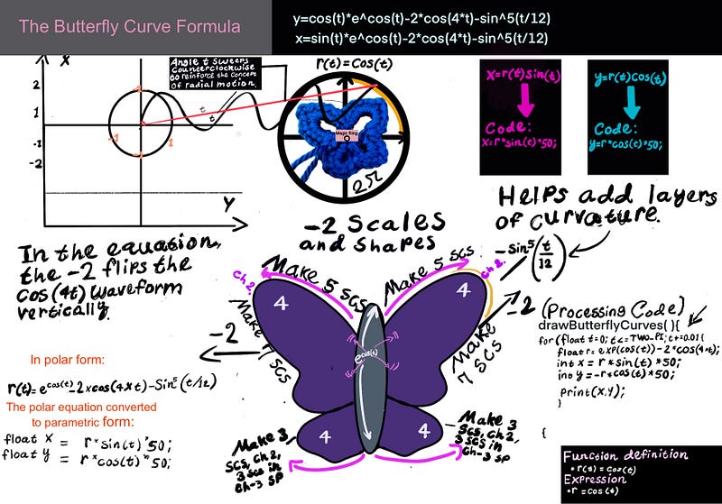
This is denoted by the equation:

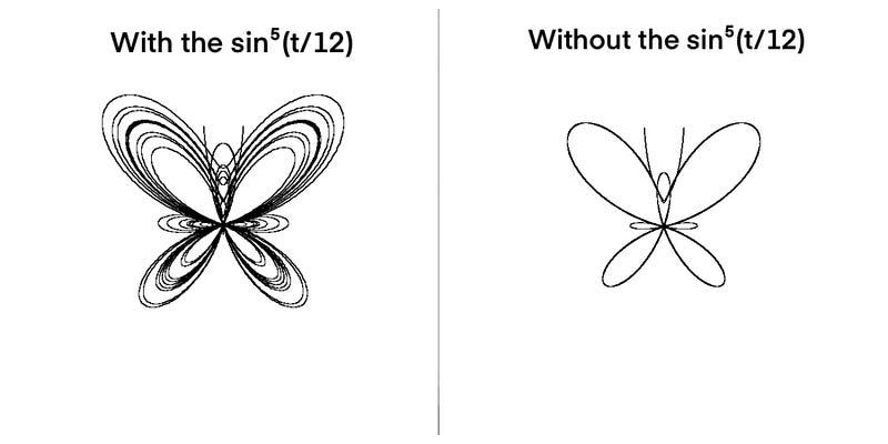
Next, we look at how the butterfly curve combines exponential growth (exp(cos(t)), symmetry from cosine oscillations (-2 * cos(4t)), and fine detailing (sin⁵(t/12)) to create a shape that grows and contracts in a consistent way across all four quadrants. These mathematical terms together allow the curve to capture the symmetrical outline of butterfly wings, with both large-scale structure and intricate detail.
You can graph the curve here on the Desmos calculator. This equation features three major parts inside the parentheses. Each term represents a different main section of the butterfly.
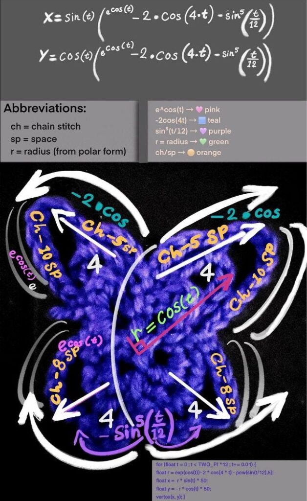
Looking at the equation from the perspective of crochet
Additionally, I thought it would be helpful to break down the equation into its respective zones on the coordinate plane. Specifically, we gain a clearer image by analyzing how the top, bottom, left, and right butterfly wings form. Then, we will examine this through the scope of a crochet project to better understand its real-life application.
1. Defining the Butterfly’s Body
The term e^cos(t) forms the central part of the butterfly anatomy. In crochet terms, it’s like creating a longer foundation chain that spans from the head down to the bottom to shape the body.
The letter e, also called Euler’s number, stands for the base of the natural logarithm. It essentially represents either growth or decay. For the butterfly curve specifically, it shows growth, acting like a volumizer of scale and adding fullness to the wings as t changes.
2. The butterfly’s amplitude and symmetry
The term –2·cos(4t) amplifies the radius and shapes the butterfly’s wingspan. It acts like a stitch multiplier, controlling how far the shape stretches from the center. The 4t factor causes the function to repeat four times over a full rotation, producing a balanced, four-lobed symmetry. The factor of 4 in cos(4t) oscillates four times over a full rotation of a circle (0 to 2π), which directly contributes to the four-lobed symmetry of the butterfly.
In crochet, this mirrors how gauge and stitch pattern define the size and structure of a motif — where repeated stitch groups shape volume and a mirrored symmetry.
3. Detailing
The term sin⁵(t/12) is the part of the equation responsible for giving our digital butterfly its detailed properties. Without this term, the butterfly would appear as a basic butterfly outline.
This part makes the butterfly wings appear fine, with the ‘ripples’ resembling ridges along the edge of each wing. This part is comparable to the detailed work created within crochet projects, such as picots, frills, or edging.
The Role of Sine and Cosine in Wing Formation
The sine (sin) and cosine (cos) functions determine the respective y and x coordinates in a way that reflects their oscillatory behavior on a Cartesian plane. This means that these functions repeat in smooth waves, like the rise and fall of a swing or ocean waves. That repeating pattern helps draw the curved and symmetrical shape of the butterfly, as the input angle (in radians) varies.
Moreover, we look a bit further into how the mathematical equation behaves within a programming environment.
Visualizing with code: Math from the angle of programming
Now that we’ve studied how mathematics shapes the butterfly curve, let’s examine how this comes to life in the Processing programming environment under the Java language. Code translates the math into motion, plotting each point as the equation unfolds over time.
The for loop sets the variable t to an incremental value of 0.01, allowing the loop to step through the equation.
Defining vs. Drawing: Polar Equations and Parametric Plots
The butterfly curve is calculated in polar form — meaning the equation tells us how far from the center to go at each angle. However, to actually draw or render the butterfly, we need to convert the polar data into x and y coordinates, which is known as the parametric form. These coordinates let us plot each point of the curve in 2D space — whether on a screen, a graph, or a crochet project.
x =  r * sin(t) * 50;
y = -r * cos(t) * 50;
Note: In Processing, the coordinate system is flipped vertically compared to the standard mathematical graphs — the y-axis increases downward from the top of the screen. As Daniel Shiffman explains in Learning Processing, this setup reflects how computer screens draw pixels from top to bottom. To account for this, we use -r·cos(t) for the vertical (Y) position instead of r·cos(t).
(float r = exp(cos(t)) - 2 * cos(4 * t) - pow(sin(t / 12), 5);Incrementing the time
The t+=0.01 in the for loop increments the angle slightly on each loop iteration, as it gradually moves through 12 complete cycles (or revolutions) around the unit circle. For t < TWO_PI * 10, the loop runs while t is less than 10 complete cycles of 2π (the usual range for periodic functions).
for(float t=0; t <TWO_PI * 12; t+=0.01){
 //Here, variables are initialized to work with the t incrementor.
}
Each cycle of 2π radians is one revolution around the unit circle, meaning the loop traces 12 revolutions (12 times around the circle). This step ensures smooth curves happen by creating many small steps. You may think of it like a spirograph tracing loops: the more revolutions, the more detailed the final shape.
In our program, two main functions represent the shape. The functions drawButterflyCurves() and drawAntennae() perform the task of drawing a butterfly shape. These functions execute in the main function void setup().
The code that renders the butterfly in Java Processing:
float x, y;
float scale = 100;
//Left butterfly Wing

//Right butterfly wing

void setup(){
  background(255); //Sets the background color of the canvas to white
  size(650,650); //Sets the width and height of the canvas

}

void draw(){
 //Moves the origin (0,0) to the center of the canvas. This is important because the rose is drawn using polar coordinates, which are centered around the origin.
  translate(width / 2, height / 2);
 //drawButterflyBody();
drawAntennae();
drawButterflyCurves();

 //ellipse(0,0,0);
}
void drawAntennae(){
  stroke(0);
  noFill();
  bezier(-1, -40, -15, -60, -25, -80, -30, -150);
  bezier(1, -40, 15, -60, 25, -80, 30, -150);
}
void drawButterflyCurves(){

  stroke(0);
  noFill();
  beginShape();
  for(float t = 0; t <TWO_PI * 12; t+=0.01){

   float r = exp(cos(t)) - 2* cos(4 * t)-pow(sin(t/12),5);
    x =  r * sin(t) * scale;
    y = -r * cos(t) * scale;
    vertex(x,y);

  }
  endShape();

}- We use beginShape() to start defining a custom shape by plotting points. This function is always paired with endShape(), and together, they wrap around the code that calculates and places each point. Inside the loop, we use vertex(x, y) to add points based on the equation, and Processing connects them in order to draw the final shape.
- Again, as described a bit earlier, the statements in the program x = r * sin(t) * 50 and y = -r * cos(t) * 50 reference the Cartesian coordinates. The negative sign in y = -r * cos(t) * 50 flips the vertical orientation of the curve.
- In Processing, the y-axis grows downward, unlike standard math graphs. The minus sign flips the butterfly right-side-up, preserving its symmetry. Without this, the butterfly would appear upside down. If we hadn’t flipped the orientation, the butterfly would appear upside down. This is because the y-axis increases downward in Processing, unlike the upward-increasing y-axis in traditional Cartesian graphs.
- Once again, the term exp(cos(t)) in the context of Processing causes the butterfly to scale dynamically, as if it’s breathing in and out—inflating and contracting along the curve. Much like how a crochet artist builds rows that expand or taper, this exponential term uses the wave-like motion of cos(t) to stretch the shape outward in some places and draw it inward in others, creating the illusion of a living, expansive form.
- Similarly, pow(sin(t/12),5))—equivalent to (sin⁵(t/12))—raises a stretched sine wave to the fifth power, smoothing valleys and sharpening peaks. This adds refined ripple-like textures to the wings. Much like decorative stitch work in crochet.
- In terms of the Bezier curve function values that set up the antennae, I suggest playing around with the values to determine what works and what doesn’t. Much of the process involves trial and error, and it’s a great way to practice!”
Program Output
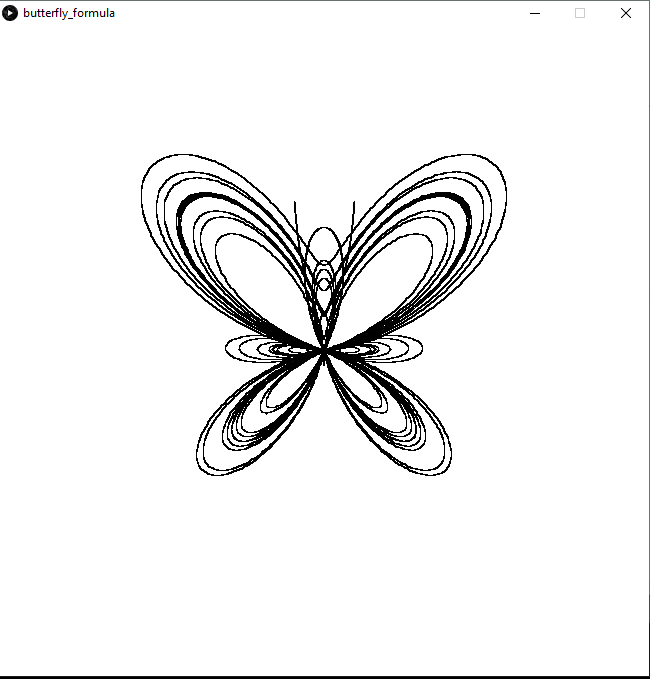
Try experimenting with the equation to see how each part shapes the curve. For example, I altered the equation slightly each time I ran the program to see what parts of it affected how the butterfly appeared.
Here, I omitted the portion of the equation responsible for detailing (sin^5 (t/12)
Translating Math Into Crochet
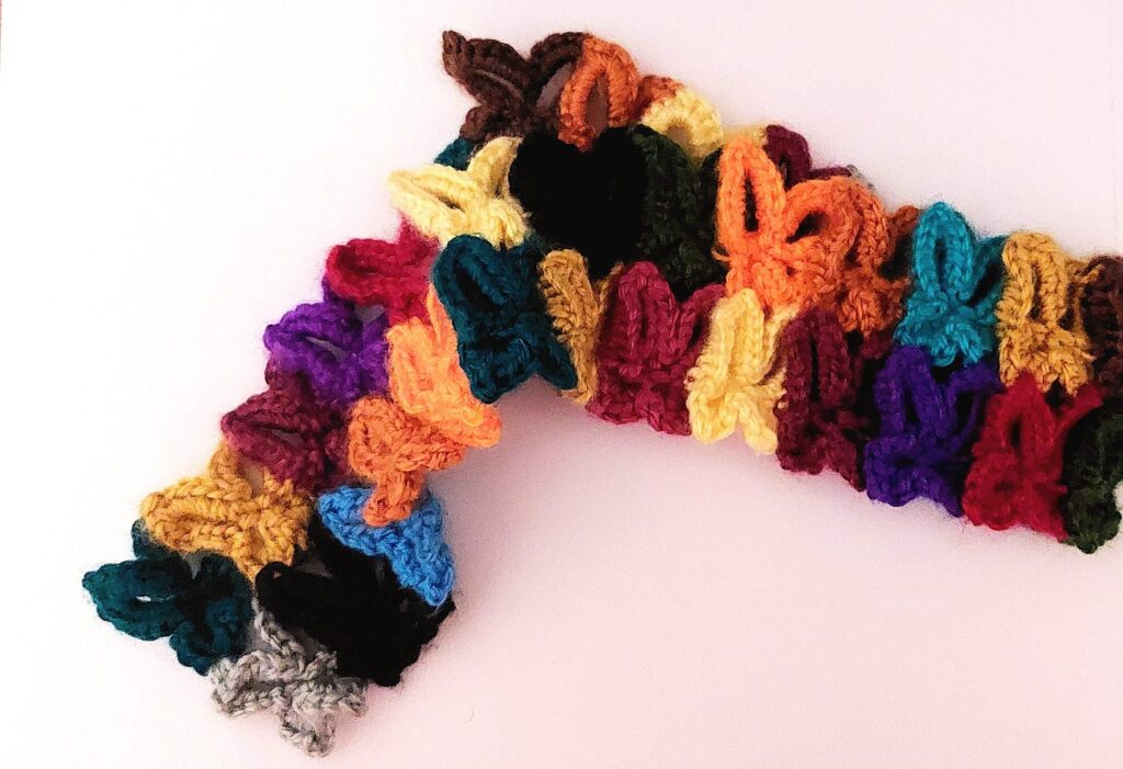
Finally, let’s take what we explored through programming a step further. Here, we duplicate the results. Only this time, those results are put into physical form as crocheted items.
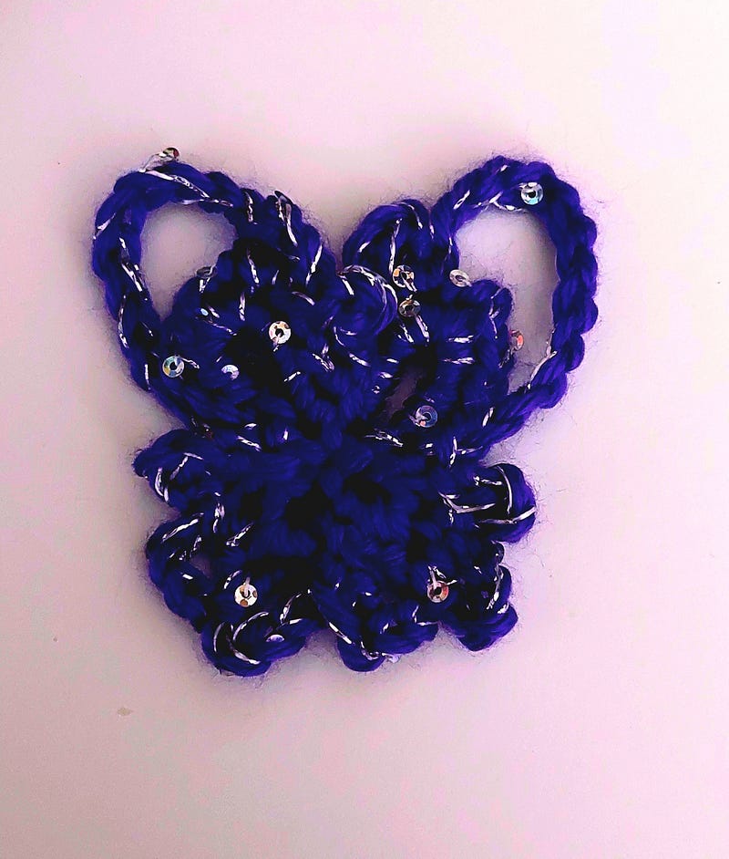
In this way, each chain and slip stitch worked from the center helps form the butterfly’s body, mirroring the central part of the mathematical curve. The larger loops extending outward represent the prominent upper wings, while the smaller loops below correspond to the shorter, lower wings.
Crocheting the butterfly appliqué
This butterfly pattern starts with a magic ring (or a chain-space, alternatively) and builds out using just chain stitches. That’s pretty much all that’s needed to create the foundational outline of the butterfly. From there, it’s all about stitch choice, shape preferences, placement, and repetition to bring the wings to life.

I use crochet abbreviations like ‘ch’ (chain) and ‘st’ (stitch) throughout this example. But if you’re new to crochet or not yet familiar with these terms, you can find a complete list of abbreviations and their meanings, Crafty Yarn Council gives a more detailed list [here].
Crochet Steps Summary:
Like the butterfly in the equation or the programming environment, the crocheted butterfly follows the same fundamental logic: repetitive instructions done in a specific order to produce a recognizable shape. In this case, our chain stitches and structured loops work as replacements for variables and other types of control flow in the program. Yet, the essence is the same.
1. Initialize the center:
Using your crochet hook and yarn of choice, start with a magic ring or a loop to define the butterfly’s core. This creates the central point from which all symmetry extends.
- Start Center: Magic ring or ch 3, join w/ sl st.
2. Create foundational loops:
We can create as many chains as needed for the bottom wings. Use these chain stitches to outline the axes of the wings. You may even think of these loops as scaffolding in the program or as the axis for the diagram.
- Lower Wings: [Ch 3, sl st into ring] × 2.
- Upper Wings: [6 sc into ch-7 sp, ch 2, 5 sc] × 2.
3. Build symmetry through repetition:
As we work our way from the center (magic ring), we fill in the wing outlines (chain spaces) by repeating any sequence of stitches with chains, single/double crochets to form the wings.
- Lower Wings: [3 sc into the ch-3 sp, ch 2, 3 sc] × 2.
- Upper Wings: [6 sc into ch-7 sp, ch 2, 5 sc] × 2.
4. Anchor at defined points:
The slip stitches or joins from previous steps create new points upon which we can anchor new stitches. They return the sequence to the center or pivot points , creating closure and reinforcing the shape.
- Anchor: Sl st between spaces that form the wings.
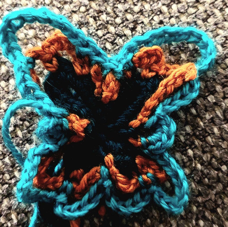
5. Add optional decorative elements:
On the third row, add more stitches and chain spaces to build upon the foundational butterfly shape. Use picots, puff stitches, frills, or shells to enhance each wing quadrant.
- Decorate (Optional): Add picots, frills, puff stitches.
6. Finalize the shape:
Secure and fasten off, optionally adding antennae or border details. The resulting form resembles a natural butterfly and a plotted figure — symmetrical, modular, and shapes the typical outline.
- Finish: Fasten off, weave in the ends, and add antennae, if desired.
Closing the Butterfly Equation
We explored how a single shape, the butterfly in this case, can transform across different contexts. Whether it is found in nature, drawn through mathematical equations, rendered in code, drawn on paper, or handmade with yarn, all versions are connected by the same underlying math.

When we look closer at the mathematical concepts playing out before us in the world and how shapes are formed, everything falls into perspective.
Let’s keep exploring together!
If you enjoyed learning about the connection between mathematics, butterflies, crochet, and code, don’t forget to follow me for more creative explorations.
❤️ Enjoyed this post?
🧶 Share with a fellow maker
✨ Follow for more math-meets-craft stories
💬 I would love to hear your perspective on this topic. Tag me or comment below
References
- Fay, T. H. (1989). The Butterfly Curve. The American Mathematical Monthly, 96(5), 442–443. https://doi.org/10.2307/2325155
- Libre Texts Mathematics. Polar Coordinates — Graphs: Goes over the different polar equations that exists other than the butterfly curve.
- Wolfram MathWorld: Provides detailed information on the butterfly curve and its mathematical properties.